
Good afternoon or good evening.


.
Cross-correlations
Observation of the cross-correlations between many pairs of series (presented as plots) can be a helpful method of the market fluctuations study. In this method plots of market shares are to be compared in selected period of time.
Those plots present stock quotes changes in time.
The examined company has a status of the base company. Its prices of shares are to be compared with other shares by calculation of correlations. As a result we get overlapping graphs, which are helpful in the prediction of the stock quotes of the basis company in the future.
Historical prices data is accesible on-line.
This data can be downloaded for instance at finance.yahoo site. One can hypothesize that the market reacting on several situations, acts in schematic way, so history repeats itself. It helps in prediction, e.g. in option pricing. However it is important to know, that any prognosis doesn't give 100% assurance.
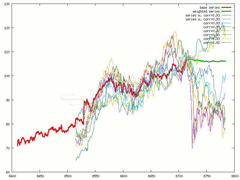
 An example of correlated series (a horizontal axis - days of trading)
During predication it is necessary to take some assumptions. The correlation is the mathematical function with codomain [-1, 1]. This codomain is referred to as a range of the correlation, but the best value referring to the highest degree of similarity is 1. To study cross-corelations of stock quotes, we chose the series with cross-correlation close to 1.00, e.g. 0.85 and higher. The choice of the series with lower correlation flattens the curve of weighted series (green line on the plot), so it makes the predication worse. Other way to get similar results is choosing of fixed amount of the best correlated stock quotes - for example 100 series.
 A result of choosing minimal correlation = 0.85
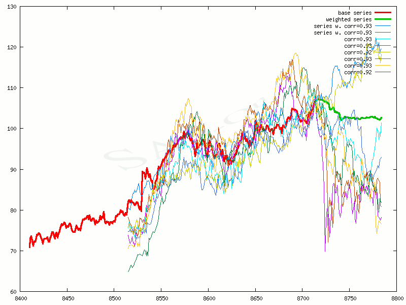 A result of choosing 100 best correlated stock quotes
There is an equation for the weighted series from points of the cross-correlated stock quotes, they are plotted by bold green line on the graph above. Every point of this bold green line is a coordinate of weighted series in time t, ie. (p, t).
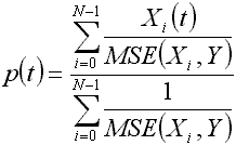 where:
N - number of series, which are taken to compute weighted series;
Y - series of the base company;
Xi - series closed to the base one, coming from the set of compared stock quotes;
MSE(...) - mean squared error between Y and Xi.
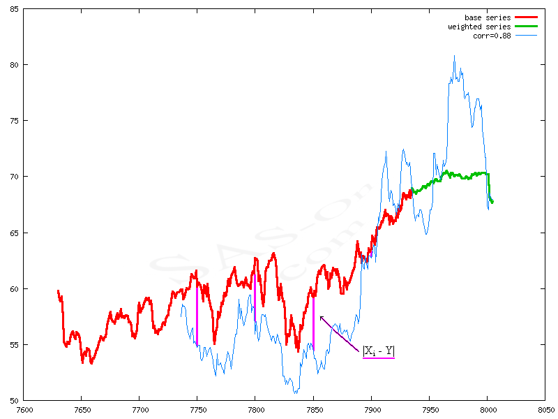 A meaning of distance |Xi - Y| - magenta lines between base series and correlated series
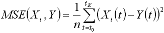 where:
n - the length of compared series, but also a period reffering to calculation of correlations;
Y - series of the base company;
Xi - series closed to the base one, coming from the set of compared stock quotes;
t0 - accepted initial value of time;
tK - accepted final value of time (length of time series resulting from tK).
Finding the same series on the stock market is almost impossible in significant period, so dispersion of curves on the graph is inevitable. This is a natural mechanism of the stock market. So the dispersion of curves after the convergence point should not be surprising. Maximum spread of curves on the graph is an extreme dispersion (the blue curves on the plot below).
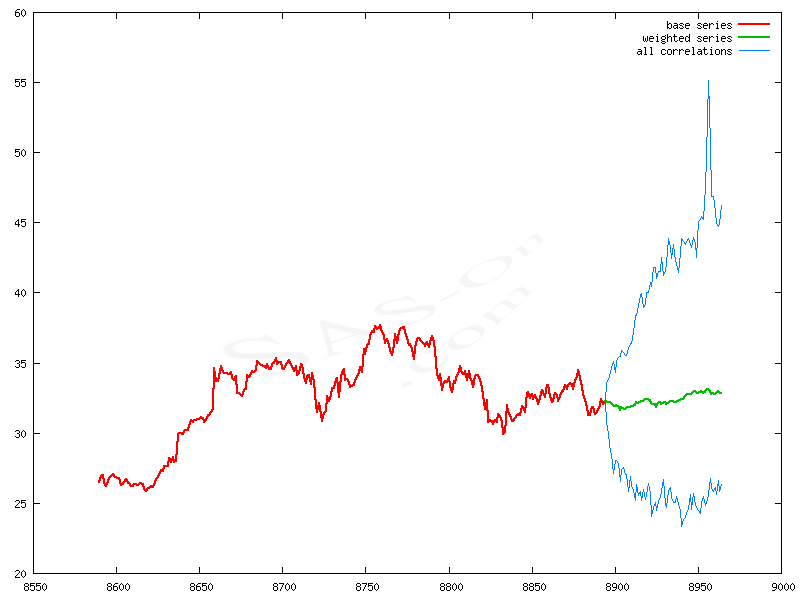 An extreme dispersion after convergence point - blue curve
Correlation has something in common with covariance (cov(...) ). Covariance is a measure of how much two random series change together. Variance is the covariance of the series with itself (this is a special case of the cov(X, X) ).
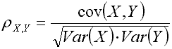 where:
ρX,Y - correlation between (time series) X and Y;
cov(X, Y) - covariance between X and Y.
Another measure of similarity is cointegration. It is harder to implement than correlations, but it can give more precise results. In this method we have to determine a confidence level (CL). In economic statistics a CL = 95% is to be determined in most often cases. When two series (Xt and Yt) are studied, one has to check if values Yt - β Xt are a white noise (i.e. random variable with a Gaussian distribution) to verify if they are cointegrated. White noise can be met in several situations, e.g. a sound of an untuned radioset. Series cointegrated in a way that hypothesis is confirmed for CL = 95% are differentiated by the white noise. In mathematical notation we get:
Yt - β Xt ∼ I(0)
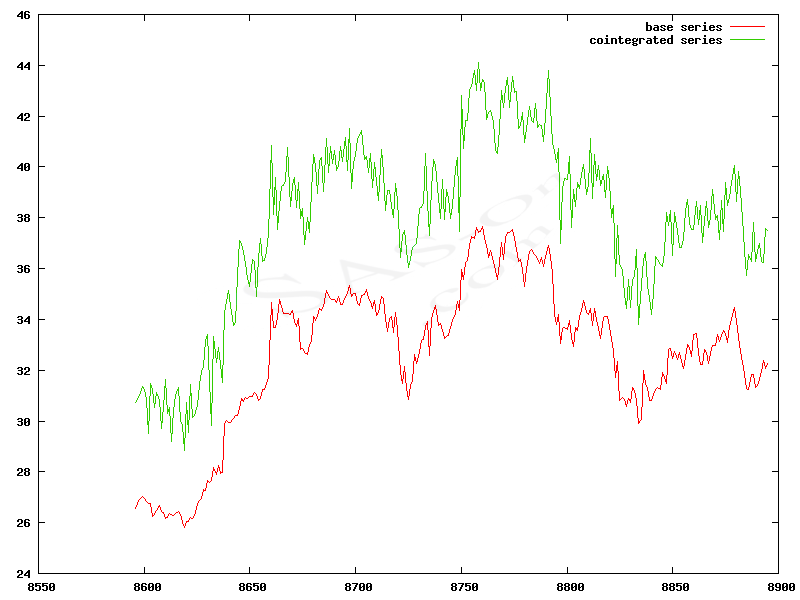 A graph of two series with cointegration = 0.86
Another example of covariance is CAPM model, which is commonly used by brokerage houses. This model shows a relation between a systematic risk of asset or of portfolio and a average rate of return. CAPM uses a covariance matrix of stock shares.
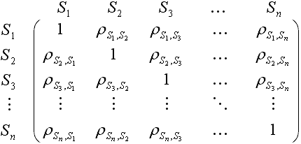
One of often used method to describe the correlations is cluster analysis. The graph of cluster analysis is known as a correlation tree. The first step of this method is to calculate a correlation matrix for time series, e.g. for S1, S2, S3, ... and Sn. We calculate correlations for every pairs of series, a correlation of series with itself is also taken into account, but it always equals 1. We get a symmetric matrix, which can be presented in the following way:
There are 3 ways to get the matrix of distances from the correlation matrix. They are described by formulas listed below, which apply to each element separately, and not the whole matrix:
1a.) dis = 1 - ρ or
1b.) dis = (1-ρ)/2
2 ) dis = 1 - |ρ |
3 ) dis = sqrt(1-ρ2)
Most often used are 1a. (when we know that correlations are only positive) and 2. (when we know that correlation values can be either positive or negative).
These methods let us get the matrix of distances. From the matrix of distances one can get a set of clusters, which creates a correlation tree. It can be solved in this way using SAS (Statistical Analysis System):
proc corr data = series outp = corrPearson noprint;run; proc varclus data = corrPearson (type=CORR) maxclusters = 309 noprint outtree = corr_tree;var _numeric_;run;proc tree data = corr_tree horizontal;id _name_;run; The result of cluster analysis done by the SAS shown above
Correlations can help, e.g. in forecasting of currency quotes in the short-term. This method helps me with decision of buying currencies. My experience tells me it is effective. One can use correlation analysis in planning of buying or selling shares. However this is only a forecast so it can not predict for instance unexpected political situation (e.g. the economy of Greece being close to collapse), natural disasters etc.
Cluster analysis can help with diversification of the portfolio to increase a potential profit with less risk. So it can be usefull when one has to make decision which shares are worth to buy or sell.
Cluster analysis can help with diversification of the portfolio to increase a potential profit with less risk. So it can be usefull when one has to make decision which shares are worth to buy or sell.
[1] Davood Rafiei, On Similarity-Based Queries for Time Series Data [in:] 15th International Conference on Data Engineering, Sydney, Australia, March 23 - 26 1999, IEEE Computer Society, Los Alamitos, California, 1999, p. 410 - 417.
[2] Harry M. Markowitz, Mean-Variance Analysis in Portfolio Choice and Capital Markets, Frank J. Fabozzi Associates, New Hope, Pennsylvania, 2000.
[2] Harry M. Markowitz, Mean-Variance Analysis in Portfolio Choice and Capital Markets, Frank J. Fabozzi Associates, New Hope, Pennsylvania, 2000.
The data send via this form will not be shared with others. When conversation will not be continued then information about e-mail will be removed automatically after 2 months.
Please take into account that connection is not secured (no https) so form data will be send as open text.
Fields like e-mail, solution of equation and any text message are necessary to complete before sending to the website owner. He is grateful for attention and for your contact.
