
Good afternoon or good evening.


.
Capital Asset Pricing Model (CAPM)
CAPM this is the mathematical model, based on the covariance matrix, which is used to examine the relation between systematic risk, and expected rate of return. This model was introduced in the sixties of 20th century by four economists independently: three Americans - William F. Sharpe (Stanford University), Jack Treynor (present President of Treynor Capital Management), John Lintner (Harvard Business School) and Norwegian - Jan Mossin (Norwegian School of Economics). Their works were based on "Portfolio Selection: Efficient Diversification of Investments" by Harry Markowitz (published in 1959). Harry Markowitz, born in 1927, received his PhD from the University of Chicago with a thesis on the portfolio theory. In 1990 he received The Sveriges Riksbank Prize in Economic Science in Memory of Alfred Nobel together with M. Miller and W. F. Sharpe.
CAPM is described by the equation below:
E(Ri) = Rf + βi ( E(Rm) - Rf)
where:
E(Ri) - expected rate of return;
E(Rm) - expected return of the market;
Rf - risk free rate (e.g. a bank deposit);
βi - expected excess asset returns.
E(Ri) - expected rate of return;
E(Rm) - expected return of the market;
Rf - risk free rate (e.g. a bank deposit);
βi - expected excess asset returns.
An ordinary investors goal is to have the maximum investment return with the minimum-risk. CAPM is a helpful tool to achieve this, but it is simplified. This theoretical model does not reflect all possible aspects of the market reality. In consideration of historical prices (data) of every instruments (shares, options, commodities etc.) on the market, one can calculate theirs spread (standard deviation, σ) and the rate of profit (E(Ri)) in the defined period to get series of points (σ, E(Ri) ). Then one can plot them on a graph with axes referring to CAPM coordinates (σ, E(Ri) ). One can also mix the portfolios assets (like deposit, some shares, currencies and some commodities, e.g. gold). This way of investment reduces the risk (makes σ being smaller) and adds more points to CAPM graph. Including more portfolios makes CAPM graph being more detailed. Connecting points on the left border of CAPM graph gives an envelope curve (the left side of the convex hull).
This curve is called the 'Markowitz bullet'. Its shape reminds a vapor cone (caused by fighter jet flying at transonic speed - about 1 Mach) or just a bullet.
This curve is called the 'Markowitz bullet'. Its shape reminds a vapor cone (caused by fighter jet flying at transonic speed - about 1 Mach) or just a bullet.
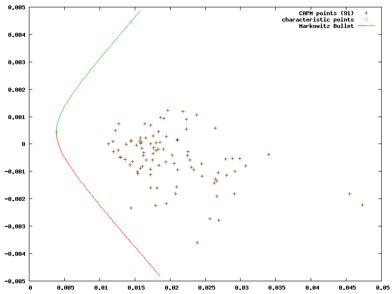 The curve called 'Markowitz bullet'
On the graph above points on the green boundary (over minimum risk portfolio point) mean the most efficient portfolios. This boundary is called the efficient frontier.
 Example of the vapor cone reminding the Markowitz bullet
(Licensed under Creative Commons Attribution-Share Alike 3.0 Unported. More here...)
On the efficient frontier one point is located extremely on the left side. This point means the minimum risk portfolio. Its variance can be estimated by the following equation:
VarCov-1⋅1'1'T⋅ VarCov-1⋅1'
where:
1' = [1, 1, 1, ..., 1]T - vector of ones - non-weighted combination of assets (ones in MatLab);
VarCov-1 - inverse of the variance-covariance matrix (another common notation is Σ-1).
1' = [1, 1, 1, ..., 1]T - vector of ones - non-weighted combination of assets (ones in MatLab);
VarCov-1 - inverse of the variance-covariance matrix (another common notation is Σ-1).
What is inverse matrix?For example a multiplicative inverse of a number 2 is 12 (or 0.5=2-1); inverse of a number 4 is 14 (0.25); for a number 5 it's 15 (0.2) etc.
System of equations can be expressed in the matrix form, for instance:
2x + 3y = 16
3x + 5y = 25
In the matrix form it looks like: To find a solution for a x, y one has to inverse the matrix of a system:
 In this example x = 5 and y = 2.
System of equations can be expressed in the matrix form, for instance:
2x + 3y = 16
3x + 5y = 25
In the matrix form it looks like:
To find a solution for a x, y one has to inverse the matrix of a system:
In this example x = 5 and y = 2.
One can get the variance-covariance matrix in the same way like a correlation matrix (described in the article cross-correlation).
First step is to compute covariances for each pair Si, Sj, where Si and Sj are a time series of assets. Covariance is a measure of how much two random series change together.
Variance is the covariance of the series with itself (this is a special case of the cov(X, X) ).
We get a symmetric matrix, which can be presented in the following way: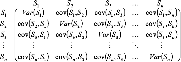
To find the Markowitz bullet, one can use Lagrange multipliers.
When this method is applied, short selling has to be accepted as a one of solutions.
Joseph Louis Lagrange (1736 - 1813) - was a mathematician and the Italian astronomer working in Prussia (Prussian Academy of Sciences in Berlin) and in France (Académie Française - French Academy). He was the first professor of the analysis at the Ecole Polytechnique.
In the CAPM method are 2 Lagrange multipliers resulting from 2 constraints, they are based on 2 assumptions:
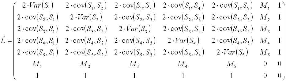
This can be expressed by general notation for any number of assets:
- one invests all capital resources, ∑ pi = 1 (where p is a vector of portfolio, or just portfolio, pi is an element of portfolio, meaning the weight of investment into the asset i; 1 stands for the fact that 100% is invested);
- an expected portfolio return (r ) chosen by the investor, expressed by the formula ∑ Mi⋅pi = r (where M is a vector of average rates of return).
This can be expressed by general notation for any number of assets:
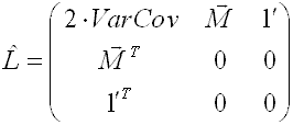
where:
VarCov - the variance-covariance matrix;
M - a vector of average rates of return;
1' - a vector of ones;
4 zeros in L (down-right corner) come from the model of Lagrange multipliers.
VarCov - the variance-covariance matrix;
M - a vector of average rates of return;
1' - a vector of ones;
4 zeros in L (down-right corner) come from the model of Lagrange multipliers.
In the Lagrange multipliers method vector on the right-hand side contains: zeros, expected portfolio return (2-nd assumption) and value 1 (1-st assumption). As a result only 2 last columns in inversed matrix of Lagrange multipliers (L) are relevant. As a result the portfolio equation has a simple linear form:
pi = L-1i,n⋅ r + L-1i,n+1
Or in programming language:
n - number of assets;
Both solutions assume that numbering starts at 0 (zero-based numbering).
for i = 0, ..., n-1 { portfolioi = inverseLi,n * r + inverseLi,n+1 }where:n - number of assets;
inverseL - inverse matrix L.Both solutions assume that numbering starts at 0 (zero-based numbering).
The next step is to compute the level of risk:
Var(p) = pT⋅ VarCov ⋅ p.
In this way one can get the Markowitz bullet point = (r, Var(p)).
Var(p) = pT⋅ VarCov ⋅ p.
In this way one can get the Markowitz bullet point = (r, Var(p)).
I use my own program to compute all portfolios. The graph in this article was plotted with its help. Using it helps me in hedging my investments.
When one compares portfolios, his own and stock index for instance, he can use Sharpe ratio. Sharpe ratio is a test of a portfolios performance in relation to its risk. It helps to evaluate the excess return. One can calculate the Sharpe ratio by division of difference between the average rates by standard deviation. It can be expressed by this equation:
E[Rp - RI]σpI
E() - expected value estimator;
Rp - analysed portfolios rate of return;
RI - reference portfolios rate of return (e.g. stock index);
σpI - standard deviation.
If Sharpe ratio is greater than 0, the result is positive (analysed portfolio is better than the reference portfolio). When one compares the portfolio to risk free rate (Rf), then the numerator is simplified to the difference between the average rate of return and Rf : E(Rp) - Rfσp
Another indicator measuring the risk of investment is aforementioned β coefficient, which means expected excess asset returns. Coefficient β is a real measure of risk - β indeed, and not the standard deviation σ, β is to measure the sensitivity of the portfolios returns with relation to market returns.
β = cov(Rp, RI)Var(Rp)
If RI represents the whole market (like the share index), then β defines the risk of portfolio to the market. Higher value of β means a chance of higher returns than the reference portfolios returns. RI can refer to company also and then β.
Investing means taking a risk. It's too risky to invest a whole capital into one share (don't put all your eggs in one basket) especially when one doesn't possess all needed information about given company. It also refers to having the same information like most of traders and not possesing illegal insider information. It is difficult to foresee the political situation also. Diversification of assets can reduce the risk. The CAPM analysis is helpful in this matter, because it can improve the investment strategy. As it was mentioned it can maximize profits and minimize the risk as well.
Harry M. Markowitz, Mean-Variance Analysis in Portfolio Choice and Capital Markets (with a chapter and program by G. Peter Todd), Frank J. Fabozzi Associates, New Hope, Pennsylvania, 1987.
The data send via this form will not be shared with others. When conversation will not be continued then information about e-mail will be removed automatically after 2 months.
Please take into account that connection is not secured (no https) so form data will be send as open text.
Fields like e-mail, solution of equation and any text message are necessary to complete before sending to the website owner. He is grateful for attention and for your contact.
