
Good afternoon or good evening.


.
Matching pursuit
Maps of matching pursuit approximation are as results of time-frequency analysis taken from transformation of input data (operand) by an algorithm (operator).
In math operand is the object of a mathematical operation. In time-frequency analysis an argument is a signal or time series like sound, Brownian motion, medical signals, stock market data etc. In matching pursuit, operand is referred to as Gabor functions, which are proposed by Dennis Gabor (1900 - 1979), who was a Hungarian physicist working in Great Britain. In 1971 he received Nobel Prize in Physics for inventing holography.
In math operand is the object of a mathematical operation. In time-frequency analysis an argument is a signal or time series like sound, Brownian motion, medical signals, stock market data etc. In matching pursuit, operand is referred to as Gabor functions, which are proposed by Dennis Gabor (1900 - 1979), who was a Hungarian physicist working in Great Britain. In 1971 he received Nobel Prize in Physics for inventing holography.
The Gabor functions are defined by[1]:
gp,q(t) = g(t-q) ei2π ⋅ p⋅ t
where t is time, p, q - fixed variables, g - fixed function with module = 1 (||g||=1), i=sqrt(-1) (imaginary unit as extension of real number to the complex number).
Matching pursuit (MP) algorithm was proposed by French scientist Stéphane G. Mallat, a professor of applied mathematics at the Ecole Politechnique in Palaiseau Codex near Paris. It was also proposed by Zhifeng Zhang, a PhD in applied mathematics at the New York University.
MP algorithm can be described by computational steps listed below:
R0 ƒ =ffor n=0, ..., N{gp,q= arg maxgi |⟨ Rn f, gi⟩|an=⟨ Rnf, gi⟩Rn+1f = Rnf - an gn}return (an, gn); Rn - it's only a notation and it doesn't mean multiplication of it as constant (scalar) and function. It is the notation for residual after n steps of calculation;N - maximum number of steps choosen arbitrarily (main task is to minimize estimation error which ensues from user settings);gp,q - Gabor function;gp,q= arg maxgi |⟨ Rn f, gi⟩| - a formula which expresses an effort to find a Gabor function being most well fitted (matched) to Rn f which is the residual left after n steps;return (an, gn) - list of coefficients paired with Gabor functions returned by an algorithm. A sum of products of the functions with coefficients minimizes estimation error.In practice it looks like that:
As already mentioned, MP algorithm can be applied to create maps of fluctuations in the stock exchange, or in other words, stock quotes. In econo-physics as well as in statistic, stock quotes used to be called data series of shares. One can extract from that data series derivations up to the limited order, such as volatility being like velocity or rate of quotes change. This volatility is ilustrated below.
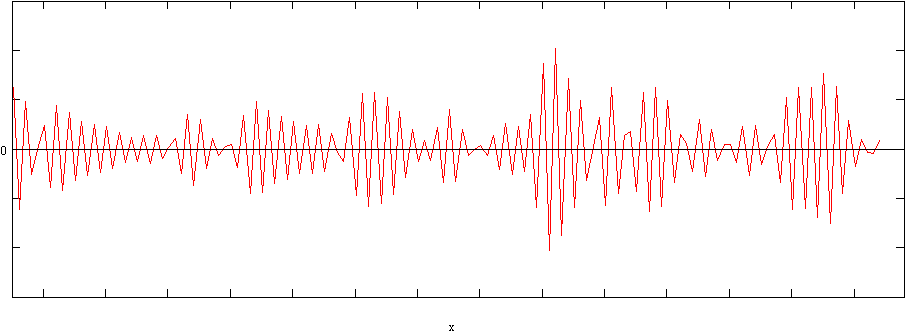 A horizontal axis - days of trading;
vertical axis - fluctuations of prices depending on previous values in data series;
the red line represents the velocity of quotes change.
The graph above presents a line having rapid changes being too fast, which seems to be chaotic, but this is an illusory impression, because several regularities of this time series can be followed easily. One can find a way to eliminate this illusory chaos - smoothing functions can be applied to achieve this. As a result we get a graph being a boundary of the red curve.
To study the signal frequency its meaningless if last value of the red curve is positive or negative. This value can be assumed initially. It is applied into first 3 methods described below. The easiest way is to apply the sign alternation (+/-) elimination. We can do it in this way:
for(i=size-1; i>0; i-=2){datai-1 *= -1;}The algorithm shown above describes multiplying by -1 every second element from the end of time series, but this is not important if there is a negative or positive value at the end of the series.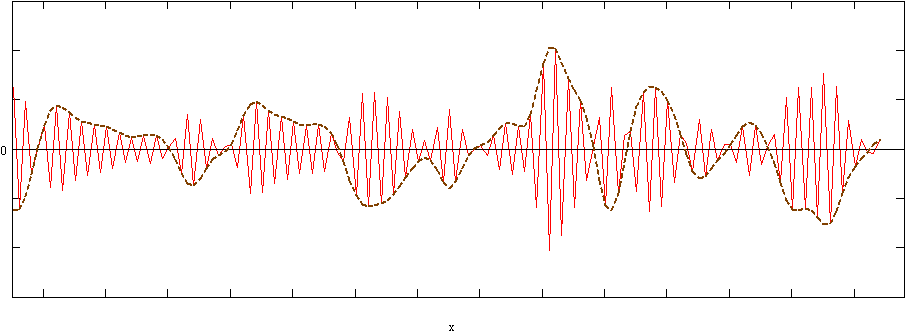
Another solution is presented as next algorithm:
d = |datasize-1|/datasize-1;sign=(d>=0.0)?1:-1;for(i=size; i>1; i--){d = datai-1/datai-2;datai-1 = datai-1*sign;if(d<0.0) sign *= -1;}This method leads to keeping the positive value at the end of the series. If we changed this line of algorithm: "sign=(d>=0.0)?1:-1;" into that one "sign=(d>=0.0)?-1:1;", then we will get a negative value at the end of time series, however if we replace "sign=(d>=0.0)?1:-1;" into "sign=1;", then we will get the initial sign at the end of time series.One "classical" method of signal processing (noise reduction) using Fourier transform (FFT), which is widely used in mathematics and physics, is inadequate in this case because it doesn't eliminate the whole problem of sign alternation.
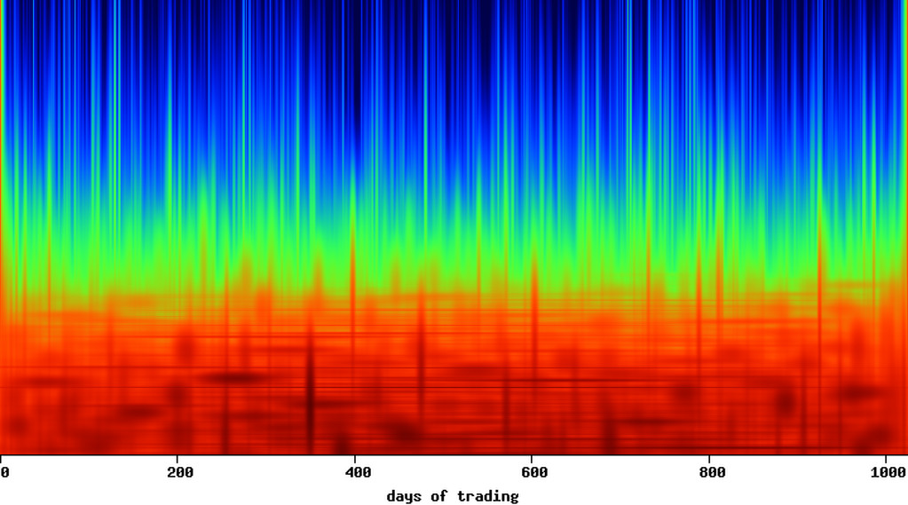
An example of a Matching Pursuit map could look like this:
How to analyse this?
This contour plot has been created using rainbow colormap: blue color means low value, red means high value. The example above shows us moments of high volatility, marked by local concentration of the red color. The results of this plotting method are dark red, vertical, sharp shapes. When MP map is applied into stock market index in selected periods of time, one can extract important information about the situation on the market or on its selected sector. Study of the history of stock market finds the existence of one interesting regularity - most of falling market trends start rapidly, but most of raising trends - mildly. When the investor finds vertical, sharp shape on the MP map, he can expect incoming falling trend (bear market). Using MP maps can be significant for the investor in planning his own stock market decisions.
The MP graphs can be applied into companies, selected or belonged to particular industry, quoted in the stock market index. Results for the selected set of companies (f.e. for market sector) have to be averaged by the weighted mean <x>w for every time-frequency coordinates. This coordinate system is significant for MP maps of the time series of companies and it can be used to compare them. It is important to notice that the MP map of every company quotations has its own weight set by rating agencies. This weight is an important factor in the weighted mean computation for the selected index or the market sector. It is not necessary to use the weight set by rating agencies, one can use the trading volume of the company at a given time as a weight (wi). This method is described by the equation below:
M(t, ω)=∑ wi⋅ mi(t, ω)∑ wi
where
M(t, ω) - weighted MP map;
t - time coordinate;
ω - frequency coordinate;
mi(t, ω) - a MP map for selected company indexed by i;
wi - a weight of company i.
M(t, ω) - weighted MP map;
t - time coordinate;
ω - frequency coordinate;
mi(t, ω) - a MP map for selected company indexed by i;
wi - a weight of company i.
The MP map being generated in this way represents results for the whole market sector or for the selected stock market index in chosen time, f.e. 1000 days.
[1] Feichtinger Hans G., Strohmer Thomas, Gabor Analysis and Algorithms: Theory and Applications, Birkhäuser, Boston 1998, p. 91.
[2] S. G. Mallat, Z. Zhang, Matching pursuit with Time-Frequency Dictionaries, IEEE Transactions on Signal Processing, 41, 12, december 1993, p. 3397-3415.
[2] S. G. Mallat, Z. Zhang, Matching pursuit with Time-Frequency Dictionaries, IEEE Transactions on Signal Processing, 41, 12, december 1993, p. 3397-3415.
The data send via this form will not be shared with others. When conversation will not be continued then information about e-mail will be removed automatically after 2 months.
Please take into account that connection is not secured (no https) so form data will be send as open text.
Fields like e-mail, solution of equation and any text message are necessary to complete before sending to the website owner. He is grateful for attention and for your contact.
